Chris Bake
- Web Based VIC
- Phase Selectable VIC
- CrayonXA (My First 9XA)
- Crossover Voltage Switch
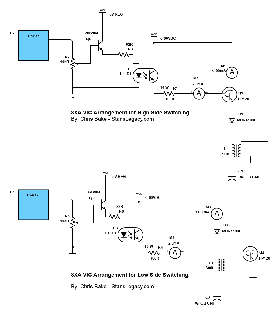
- 8XA Alternator Setup
- DIY EMF Detector
- Magnetic Amplifiers
- Saturation Oscillator
- Magamp LFO standing wave oscillator
- Introducing harmonics into Amplitude Modulation
- Bubbles
- 4 Channel 12AX7 Toroidal Amplitude Modulator
- 12AX7 Dual Triode operating in Heptode Mode
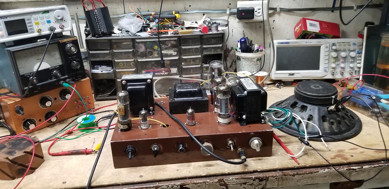
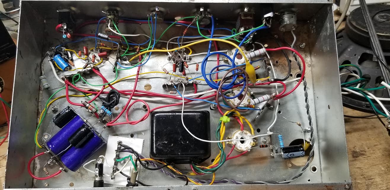
- 50W PushPull Tube Amp for driving a VIC
- Arduino / ESP32 Projects
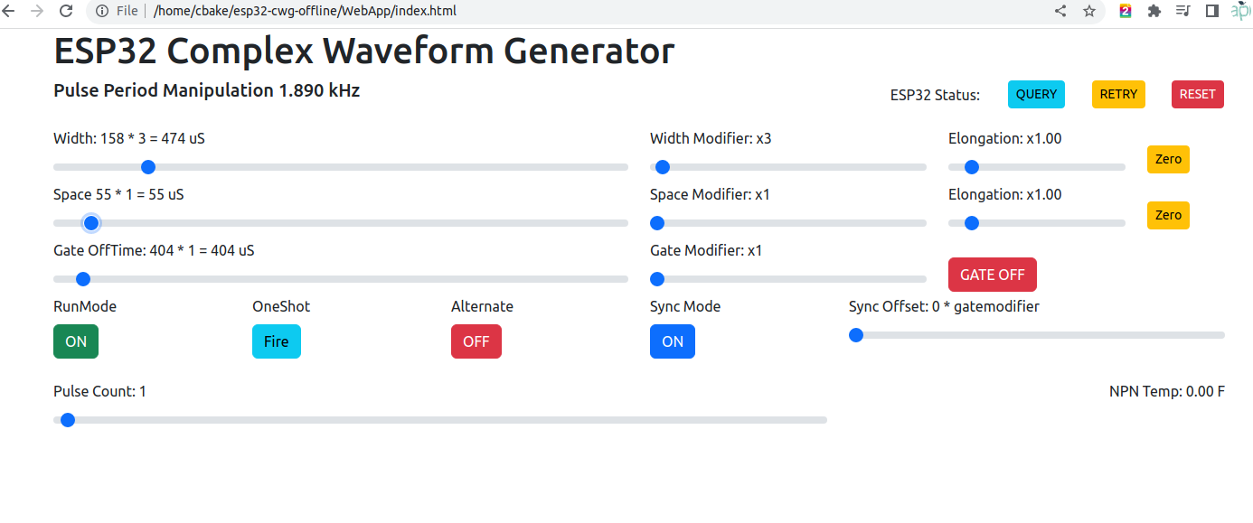
- ESP32 - Complex Waveform Generator V2
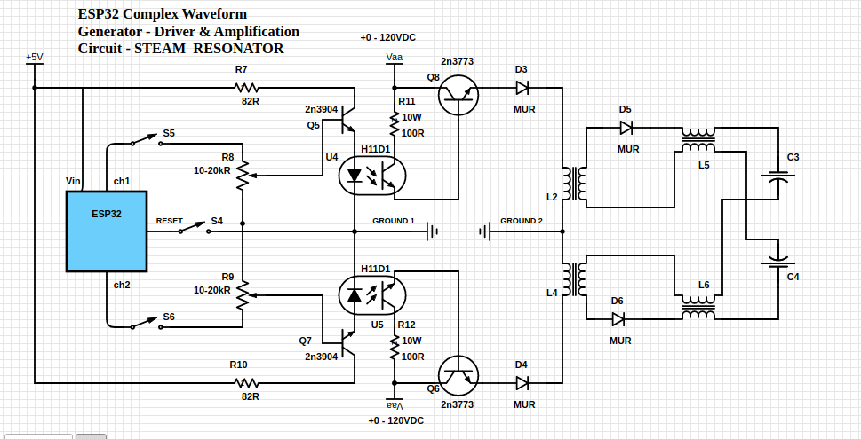
- ESP32 - CWG Driver & Amplification
- ESP32 - Complex Waveform Generator V3
- 2 Arduino - Dual Channel - Triple AND Gate (Perfect Pulse Driver)
- Core Permeability
- Resonant Modes in a Water‑Fuel Cell
- AI Conversations
Web Based VIC
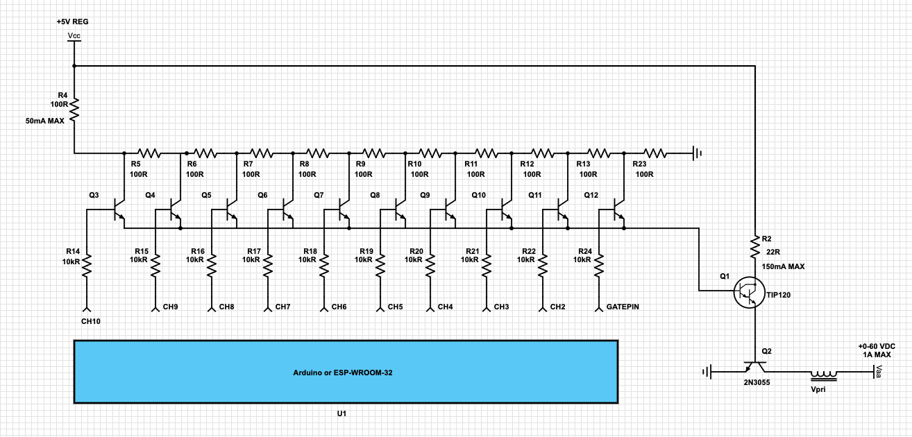
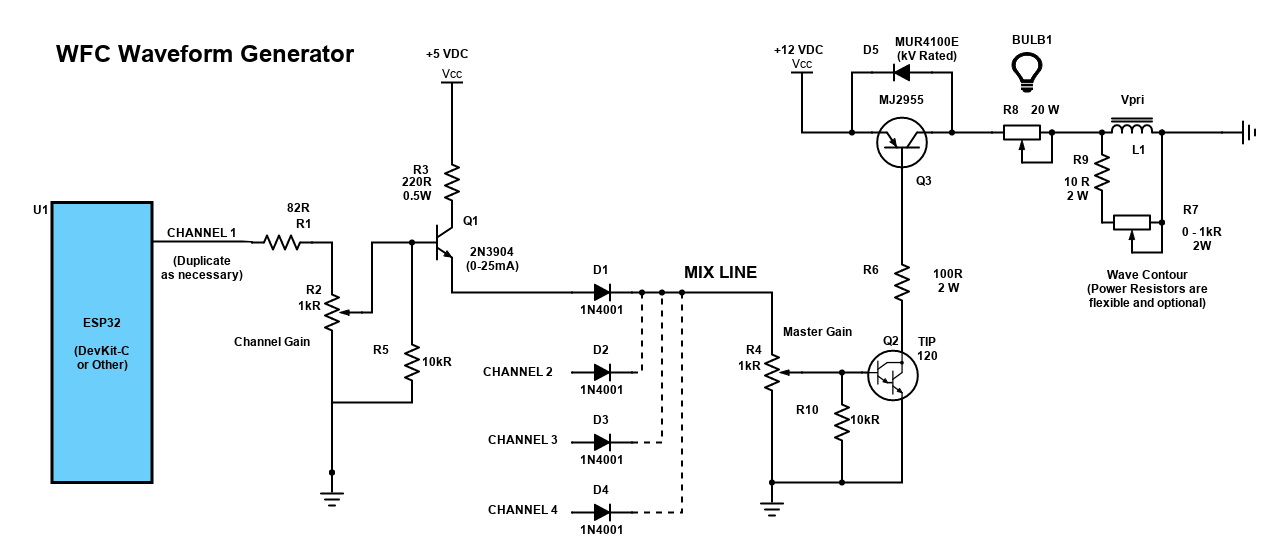
1-10 Channel Analog Amplitude Modulator
ESP32 Rest API, Pulse Clock & VIC Configurator
Phase Selectable VIC
Utilizing DPDT toggle switches to allow inline phase inversion of each VIC component allow significant selectivity in operational configurations.
450VDC push-pull EL34 vacuum tube driven VIC 4:1 stepdown ferromagnetic core
Earlier version of above, but with an added DPDT relay driven by a 3rd signal input and darlington driver, attempting the Crossover Voltage Switching utilized in the Steam Resonator.
With the monster transformer in there, I would get a very strange buildup of electrostatic vibrations on the metal chassis. No vibrations were felt on the plastic of the meter panels, but everywhere on the metal parts.
CrayonXA (My First 9XA)
Learning transistors, power supplies, 555 timers, Schmidt Triggers, AND gates, darlington transistors and optocouplers all in one shot. It still amazes me this ever worked :)
The circuit for this design originated from Max Miller's 9XA (drawn in crayon)
 |
 |
 |
A funny video illustrating how I still had much to learn about building circuits :)
More progress on the 9XA. Learning how proper transistor biasing and loading is important for controlling amplitude modulation.
Crossover Voltage Switch
8XA Alternator Setup
This was an old attempt at using an unrectified alternator's 3 phase output running from a 1/3 HP AC synchronous motor.
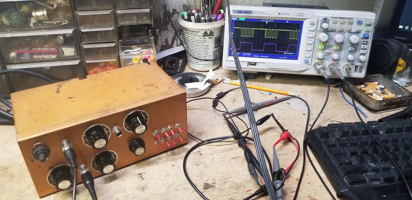
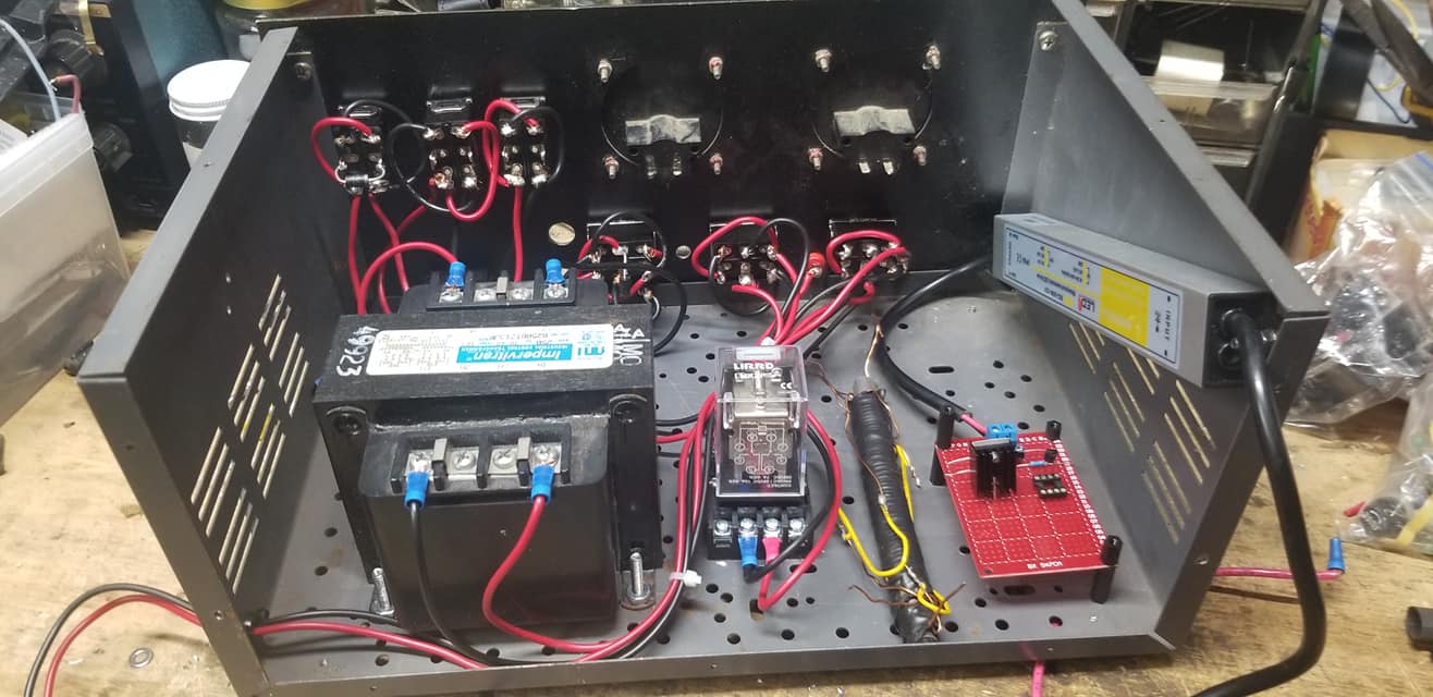
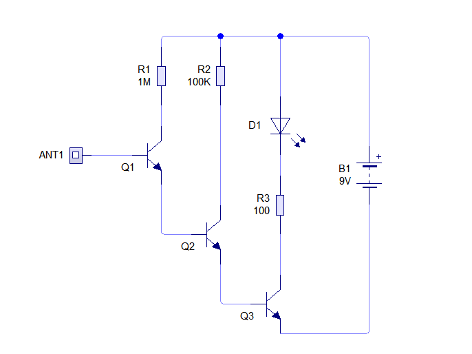
DIY EMF Detector
Easy homemade EMF probe. I added a piezo buzzer to mine, and found it very helpful to "listen" to the fields coming off of things like wires and HV bulbs, and water capacitors.
DIY Guide: https://www.instructables.com/Make-a-Ghost-Detector/
Magnetic Amplifiers
Saturation Oscillator
You must listen to your energy. It plays notes. Once you learn to trigger those notes, you can play a chord.
Playing with distributed inductances and capacitances and harmonics generated from 60 Hz line noise. Using resistive dampening to load mutually coupled transformers inline with the magnetic amplifier's reactive side.
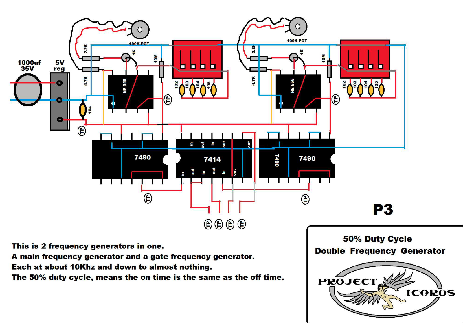
Magamp LFO standing wave oscillator
Introducing harmonics into Amplitude Modulation
Bubbles
Everything Vibrating in a WFC
This shows Max's Double Barrel cell holder adapted to mount electrodes at opposing ends of each tube.
Tiny streams of nanobubbles can be seen coming from the bolt threads
Demonstrating High Voltage present at the WFC
"Waterless" energy transfer
Visualizing standing waves occurring across the WFC capacitor.
4 Channel 12AX7 Toroidal Amplitude Modulator
Early Build pics of the 4 Channel modulator.
 |
 |
 |
 |
12AX7 Dual Triode operating in Heptode Mode
Truly Analog Amplitude Modulation AND Gating
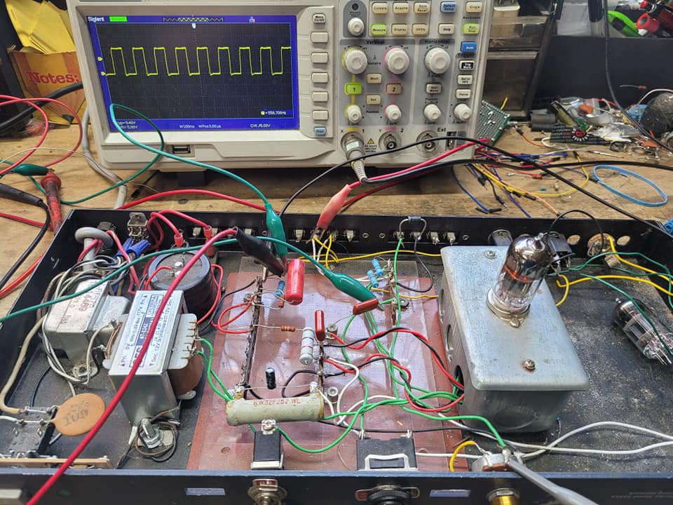
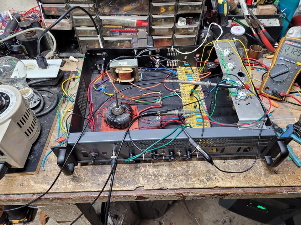
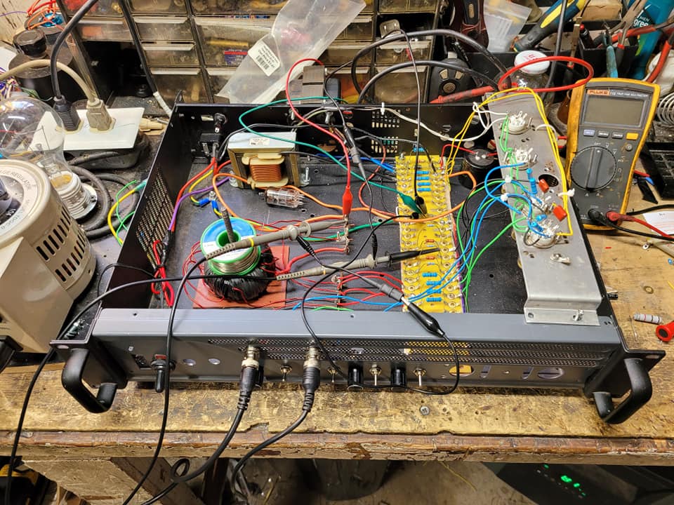
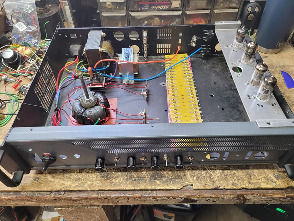
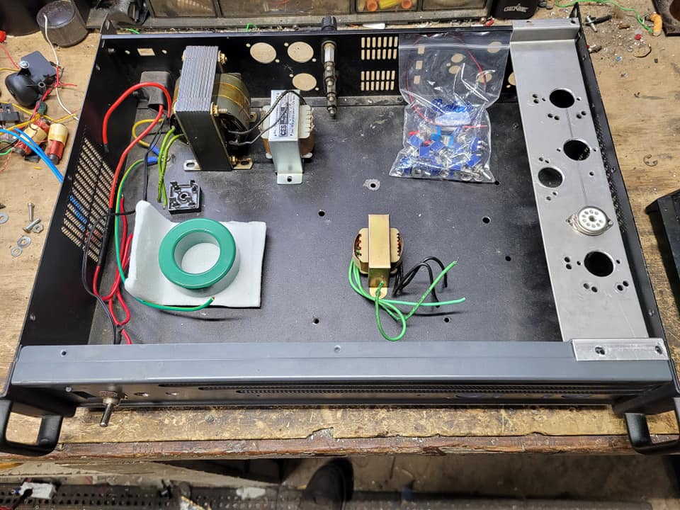
50W PushPull Tube Amp for driving a VIC
Arduino / ESP32 Projects
ESP32 - Complex Waveform Generator V2
Setting Up The App
ESP32 Complex Waveform Generator - Arrangement for WROOM-32 or WROVER-E (DevKit-C)
PARTS Required
- 1 - ESP32 (WROOM-32 or WROVER-32) with 16 exposed pins
- 1 - ESP32 Breakout Board or equivalent pin header block
- 7 - Rotary Encoders (i.e. KY-040 Rotary Encoder Module CYT1062)
- TODO: add >= 2 more for Elongation adjustments.
- 1 - +5VREG 1A Power Supply for ESP32 (i.e. ATX PowerSupply)
Installation Prerequisites
Install ESP Libraries in Arduino-IDE v2.0
ArduinoJson
ESP32Encoder
Step 1. Open Esp32Full.ino and set Wifi Credentials
// #### Change Me - Local Wifi Info ####
const char *SSID = "NETGEAR";
const char *PWD = "12345678";
Step 2. Configure free local LAN IP address
Check your Router for more information
// #### CHANGE ME ####
// Set your Static IP address to a free IP in your local network
IPAddress local_IP(192, 168, 1, 8);
// Set your Gateway IP address
IPAddress gateway(192, 168, 1, 1);

IPAddress subnet(255, 255, 255, 0);
IPAddress primaryDNS(8, 8, 8, 8);   //optional
IPAddress secondaryDNS(8, 8, 4, 4); //optional
Step 3. Configure ESP_HOST in Javascript File
Edit `./assets/espwavegen.js` and set the IP address used in Step 2 above.
TODO: Make configurable in the web interface
Save and close the file
Step 3. Upload The code in `Esp32Full.ino`
Paste the code into your Arduino-IDE and upload it to your ESP32
Installing the ESP32 Board in Arduino IDE
Step 4. Access the WebApp in your Web Browser
Open Web Browser
Open `index.html` in the `WebApp` directory below this file
- File -> Open -> Browse to WebApp/index.html -> Open
Interface is now displayed!
Step 5: Enjoy!!
Please post pics and videos of your waves, and let others know how achievable this is!
Need Amplification?
See: ESP32 - Complex Waveform Generator - Driver & Amplification
Additional Troubleshooting / Customization
Optional: Configure alternate Output Pins
- Output will be on Pins D2 and D4 by default
// #### Output Pins ####
int pinChannel1 = 2;
int pinChannel2 = 4;
Optional: Adjust Encoder Pins if needed
int pulseCount_EncoderPIN1 = 14;
int pulseCount_EncoderPIN2 = 13;
int pulseWidth_EncoderPIN1 = 35;
int pulseWidth_EncoderPIN2 = 34;
int pulseSpace_EncoderPIN1 = 19;
int pulseSpace_EncoderPIN2 = 18;
int gate_freq_EncoderPIN1 = 22;
int gate_freq_EncoderPIN2 = 23;

int pulseWidthModifier_EncoderPIN1 = 27;
int pulseWidthModifier_EncoderPIN2 = 26;
int pulseSpaceModifier_EncoderPIN1 = 5;
int pulseSpaceModifier_EncoderPIN2 = 32;
int gateModifier_EncoderPIN1 = 25;
int gateModifier_EncoderPIN2 = 33;
ESP C+ Code
Git Repo: https://bitbucket.org/cbake6807/esp32-complex-waveform-generator/src/master/
Troubleshooting:
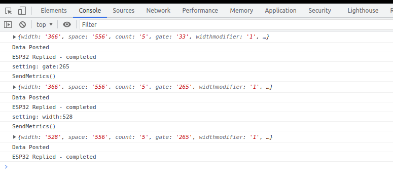
View the Console Log for errors in your browser while clicking the app's sliders buttons etc..
Look in the Network tab for red errors. 404 or other. Sometimes the ESP may drop or reject the connection on the first attempt. Just refresh the browser once or twice and it should resolve.
Confirm the ESP is a connected host in your network and was given the IP you specified
https://www.wikihow.com/See-Who-Is-Connected-to-Your-Wireless-Network
Code notes if internet connectivity isn't an option. Also, encoder wiring connections for this particular setup (Notepad++ document file type). Chris Bake ESP32 notes.txt
Notepad++ download: Notepad++
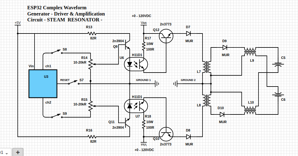
ESP32 - CWG Driver & Amplification
A dual channel, dual isolated power supply, pulse amplification for driving all VIC arrangements
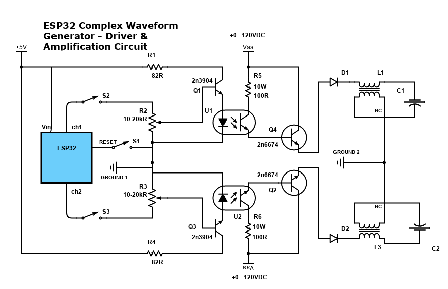
Arrangement favoring Particle Oscillation as an Energy Generator
Variation 2 - Ground Bonded / "Forced" Uni-polar Operation
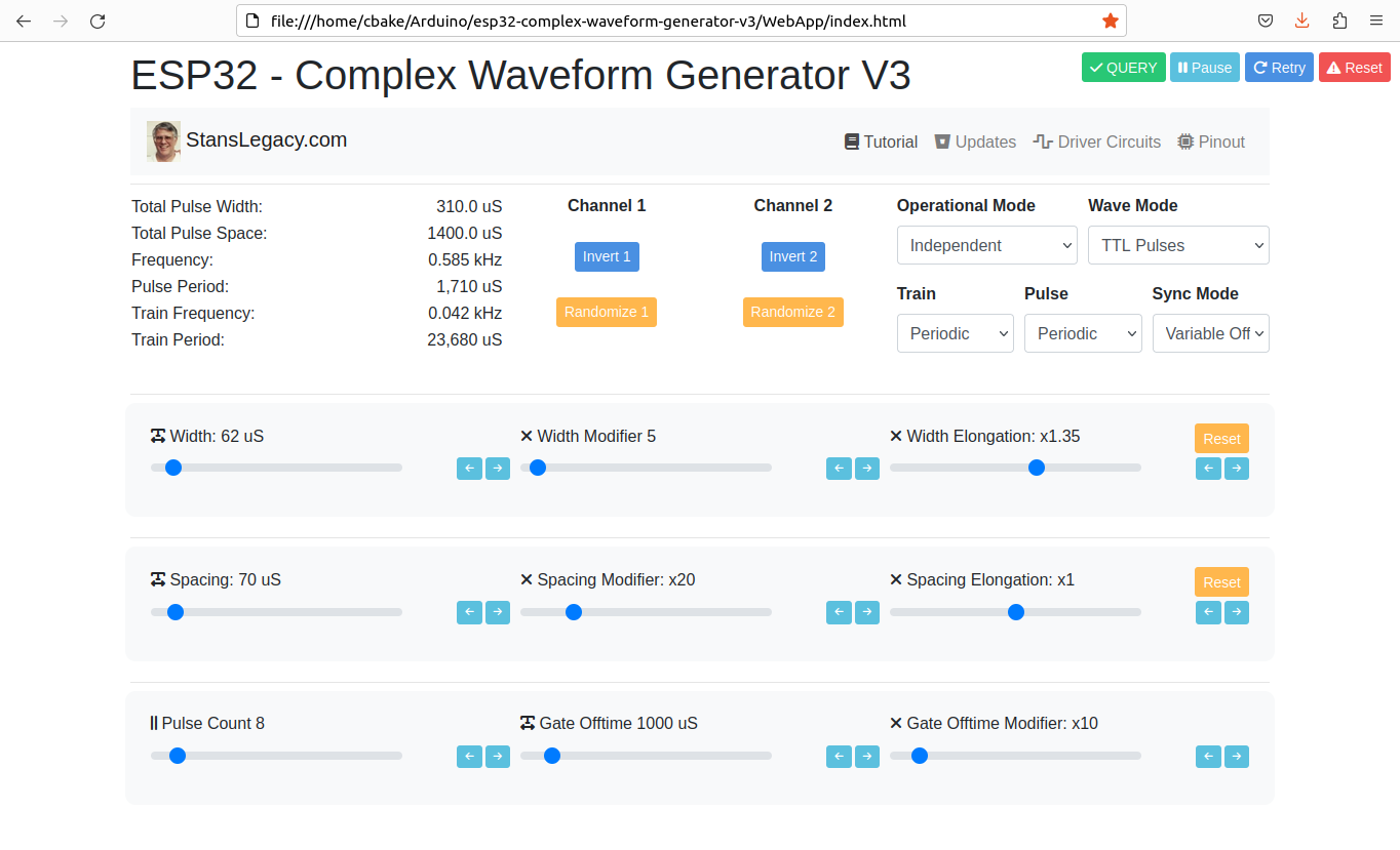
ESP32 - Complex Waveform Generator V3
Installing and Using the ESP32 Complex Waveform Generator V3 Application
Screenshot of web interface
 |
 |
Prerequisites
To use this application, you need to have the Arduino IDE installed on your computer. You can download the Arduino IDE from the official website: https://www.arduino.cc/en/software
-
ESP32 Development Board: You'll need an ESP32 development board, such as the popular ESP32-DevKitC or ESP32-WROOM-32D. These boards typically come with Wi-Fi and Bluetooth capabilities and a variety of GPIO pins for interfacing with peripherals.
-
Rotary Encoders: To adjust the waveform parameters, you will need a total of 7 rotary encoders. You can use KY-040 rotary encoder modules or any other type of incremental rotary encoder with built-in push buttons. Ensure that the rotary encoders you choose have a CLK, DT, and SW (push button) pinout.
-
Breadboard and Jumper Wires: A breadboard and jumper wires are required to make the necessary connections between the ESP32 development board and the rotary encoders.
- Power Supply: You will need a power supply to power the ESP32 development board. This can be a USB power supply, a battery, or any other suitable power source that meets the board's voltage and current requirements, such an ATX Supply from a computer. 5VDC 1A minimum is recommended to prevent brownout conditions while interacting with a driver circuit.
-
Oscilloscope (optional): To visualize the generated waveform, you can use an oscilloscope. Connect the output pins (channel1OutputPin and channel2OutputPin) from the ESP32 development board to the oscilloscope's input channels.
Installing required libraries
-
ArduinoJson: To install the ArduinoJson library, follow these steps: a. Open the Arduino IDE. b. Click on
Toolsin the menu bar, thenManage Libraries. c. In the Library Manager window, search for "ArduinoJson" in the search bar. d. Find "ArduinoJson by Benoit Blanchon" in the search results and click on theInstallbutton. -
ESP32Encoder: To install the ESP32Encoder library, follow these steps: a. Open the Arduino IDE. b. Click on
Toolsin the menu bar, thenManage Libraries. c. In the Library Manager window, search for "ESP32Encoder" in the search bar. d. Find "ESP32Encoder by Gil Mora" in the search results and click on theInstallbutton.
Uploading the Application
- Download the source code for the ESP32 Complex Waveform Generator V3 application or copy it to a new file in the Arduino IDE.
- Connect the ESP32 development board to your computer using a USB cable.
- In the Arduino IDE, select the appropriate board and port under
Tools>BoardandTools>Port. - Click on the
Uploadbutton (right-facing arrow icon) in the Arduino IDE to compile and upload the application to the ESP32 development board.
Hardware Setup
- Wire the rotary encoders and other components according to the pin assignments defined in the source code.
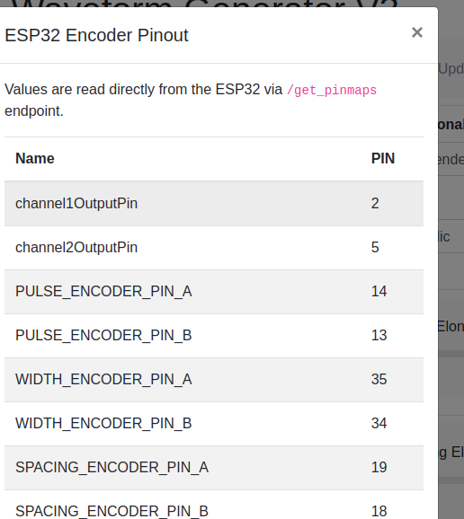
ESP32 Pin Encoder Connection Encoder Function 14 Pulse Encoder CLK Pulse count 13 Pulse Encoder DT Pulse count 35 Width Encoder CLK Pulse width 34 Width Encoder DT Pulse width 19 Spacing Encoder CLK Pulse spacing 18 Spacing Encoder DT Pulse spacing 23 Off-time Encoder CLK Off-time 22 Off-time Encoder DT Off-time 27 Width Mod Encoder CLK Width modifier 26 Width Mod Encoder DT Width modifier 15 Spacing Mod Encoder CLK Spacing modifier 32 Spacing Mod Encoder DT Spacing modifier 33 Off-time Mod Encoder CLK Off-time modifier 4 Off-time Mod Encoder DT Off-time modifier 2 Output Channel 1 Output waveform 5 Output Channel 2 Output waveform - Make sure the connections are secure and verify the CLK/DT pins for each encoder are wired correctly, and that each encoder turns in the correct direction relative to the respective parameter change.
Using the Application
- Power on the ESP32 development board.
- Use the rotary encoders to adjust the following parameters:
- Pulse count
- Pulse width
- Pulse spacing
- Off-time
- Width modifier
- Spacing modifier
- Off-time modifier
- The application will generate a complex waveform based on the adjusted parameters.
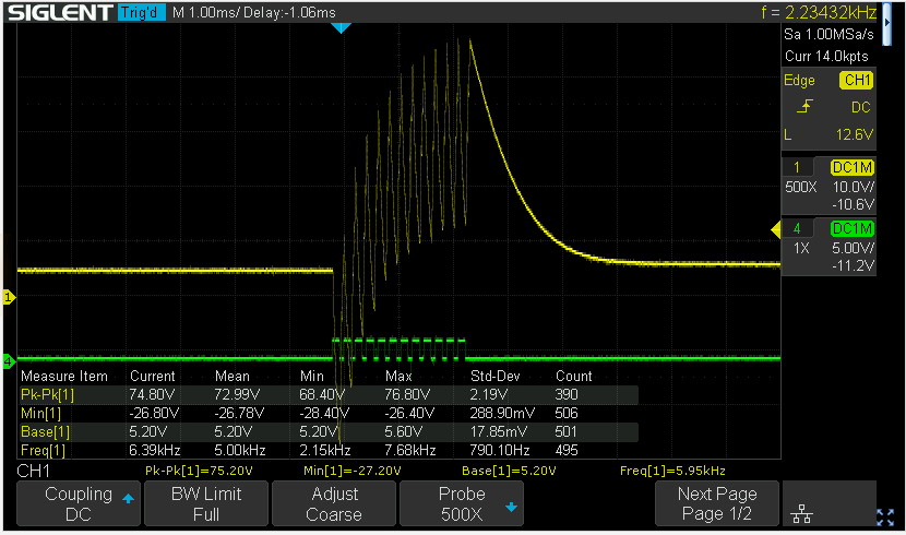
- Connect the output pins (channel1OutputPin and channel2OutputPin) to an oscilloscope to visualize the generated waveform.
- Open the WebApp/index.html page in a browser.
- Fine-tune the parameters using the rotary encoders to achieve the desired waveform shape and characteristics.
Next Steps For Utilization
- Build ESP32 CWG - VIC Driver circuit(s) - https://stanslegacy.com/books/chris-bake/page/esp32-cwg-driver-amplification
- Cell Construction - https://stanslegacy.com/books/ethan-crowder/page/resonant-cavity-related
Troubleshooting
- If the waveform does not match the expected output, verify the wiring connections and ensure the rotary encoders are functioning correctly.
- If the application does not upload to the ESP32 development board, double-check the board and port selection in the Arduino IDE.
- If the rotary encoders behave unexpectedly (e.g., adjusting one parameter affects another), check the CLK/DT pin assignments and wiring.
-
Click the PInout button to fetch the currently defined GPIO pins from the ESP32 directly and confirm they are wired correctly.

For further assistance or to report any issues, contact the application's support team or refer to the community forums.
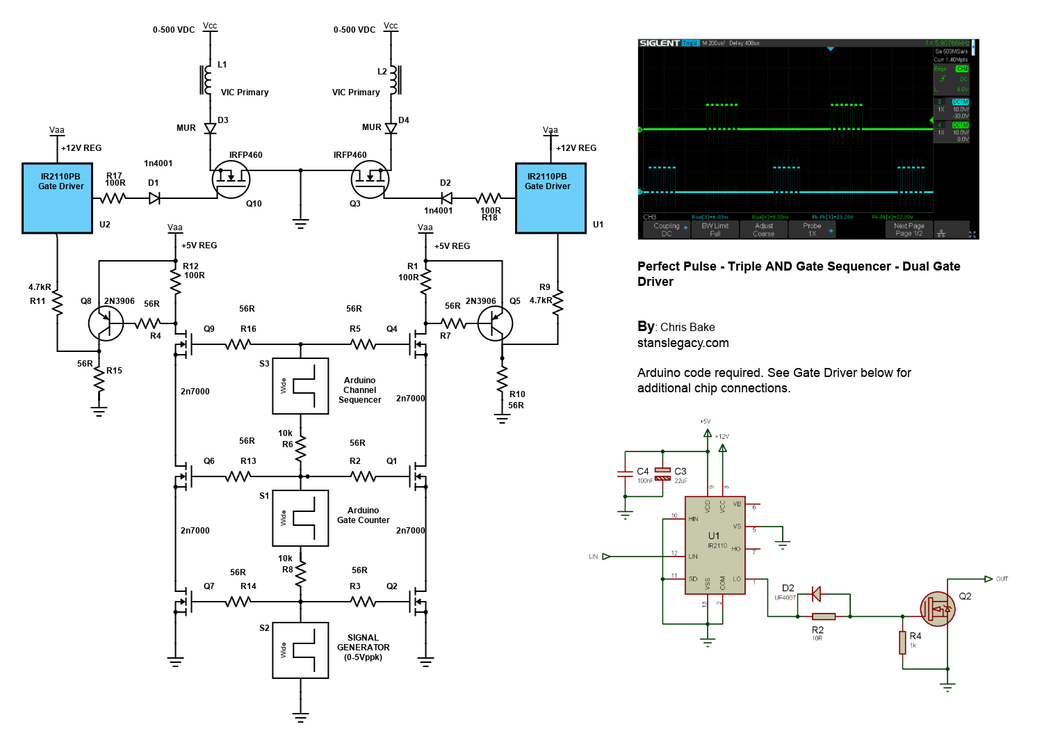
2 Arduino - Dual Channel - Triple AND Gate (Perfect Pulse Driver)
By: Chris Bake
Arduino Code: https://bitbucket.org/cbake6807/dualtripleseq/src/master/
Parts List
- External Signal Generator: 0-5Vppk output.
- Power Supply: ATX is ideal, providing +5V REG and +12V REG.
- 2N7000 Signal MOSFETs: Quantity 6.
- IRFP460 or Similar Power N-channel MOSFET: Quantity 2.
- 56Ω 1/8W Resistors: Quantity 10.
- 100Ω 1/2W Resistors: Quantity 2.
- 4.7kΩ Resistors: Quantity 2.
- 2N3906 PNP General Purpose Transistor: Quantity 2 (can be substituted with any general PNP transistor).
- IR2110PB Gate Driver Chip 14-pin: Quantity 2.
- Arduino Nano (or similar): Quantity 2 (must support hardware PCNT).
- Rotary Encoder: Quantity 1.
Software Requirements
- Arduino IDE: Ensure it is installed and updated to the latest version.
- Encoder Library: Install via the Arduino Library Manager.
Arduino Setup
Pulse Counter Arduino
-
Upload Script
- Open the Arduino IDE.
- Connect the first Arduino (PulseCounter) to your PC.
- Open
PulseCounter.inofrom the provided file. - Upload the script to the Arduino.
-
Connect the Encoder
- Connect the encoder's VCC to the Arduino's 5V pin.
- Connect the encoder's GND to the Arduino's GND pin.
- Connect the encoder's CLK and DT pins to two digital pins on the Arduino D2 and D3.
- Connect the encoder's Button pin to D4.
-
Verify Encoder Output
- Open the Serial Monitor in the Arduino IDE.
- Rotate the encoder and check the output to confirm it is functioning correctly.
const int outputPin = 9;const int encoderPinA = 2;const int encoderPinB = 3;const int encoderSwitchPin = 4;const int disableSwitchPin = 6;
Adding a Pushbutton for Sync Mode Toggle
Parts Required
Hardware Connections
-
Connect the Pushbuttons
- NANO1 - D6 -> BUTTON -> GND
- NANO2 - D4 -> BUTTON -> GND
Summary of Connections
Sequencer Arduino
- Upload Script
- Disconnect the PulseCounter Arduino and connect the second Arduino (Sequencer) to your PC.
- Open
Sequencer.inofrom the provided file. - Upload the script to the Arduino.
Pin Mapping and Connections
Connecting the Two Arduinos
-
PulseCounter Arduino to Sequencer Arduino
- Signal Generator (+5Vppk max) →PulseCounter NANO1 - D5 (Input)
- Signal Generator (+5Vppk max)→Q2 First 2N7000 FET Gate
- Signal Generator (+5Vppk max)→Q7 First 2N7000 FET Gate (opposite branch)
- PulseCounter NANO1 - D9 (Output) → Sequencer NANO2 - D2 (Input)
- PulseCounter NANO1 - D9 (Output) → Q1 Second 2N7000 FET Gate
- PulseCounter NANO1 - D9 (Output) → Q6 Second 2N7000 FET Gate (opposite branch)
- Signal Generator (+5Vppk max) →PulseCounter NANO1 - D5 (Input)
-
Sequencer Arduino Outputs
- Sequencer NANO2- D9 (Output) → Input to Q4 - Third 2N7000 Gate.
- Sequencer NANO2 - D10 (Output) → Input to Q9 - Third 2N7000 Gate (opposite branch)
- Gate Enable/Disable Button
- Connect NANO1 - D6 -> BUTTON -> GND
- SyncMode / Offset Mode Button
- Connect NANO2 - D4 -> BUTTON -> GND
Note: The schematic shows the outputs merged due to limitations, but there should be dual outputs from the sequencer, D9 and D10, each connecting to a separate AND gate tree.
Gate Driver Chip Connections
IR2110PB Gate Driver Chip
-
Power Connections
- VCC (Pin 3) → +12V REG
- VSS (Pin 2, 10, 11, 15) → GND
- VDD (Pin 9) +5V REG
-
Input Connections
- LIN (Pin 12) → Arduino PWM pin (as per script)
-
Output Connections
- LO (Pin 1) → Gate of the IRFP460 MOSFET
-
Bootstrap Capacitor
- Connect a 22µF and a 100nF capacitor near VDD (Pin 9) and Ground.
- No Connection
- Pin 6, 7 - NC
-
Noise Filtering
- R2: Connect a 10Ω resistor between LO and the gate of the MOSFET.
- D2: Place a 1N4001 diode in parallel with the Resistor R2 in reverse direction for added noise filtering and protection.
Schematic Overview
Refer to the schematic image to visualize these connections. The IR2110PB gate driver chips control the IRFP460 MOSFETs, enabling high-power switching of the VIC (Voltage Intensifier Circuit) primaries.
Additional Notes
- Resistor Tolerances: The resistors can have a large tolerance. The 56Ω value is selected to preserve signal clarity. Any value ≤220Ω should be acceptable.
- Merged Outputs: The Arduino Channel Sequencer has 2 outputs shown merged due to Scheme-It limitations.
Core Permeability
There are 2 inductors on a ferrite core, closed loop U shape. The core's permeability is approx 2000. One coil is 300 turns of 22Ga wire, and the other coil is 1000 turns of 30Ga wire. The inductance of the 300 turn coil, while shorting the 1000 turn coil, is 12.188mH. The inductance of the 1000 turn coil, while shorting the 300 turn coil, is 159.69mH. Both measurements were taken at a 1 kHz test frequency with an LCR meter.
What is the true core permeability?
We can use the following equation to calculate the inductance of an inductor on a closed loop ferrite core with two coils:
L_total = μ * N_1^2 * A / (2 * l) + μ * N_2^2 * A / (2 * l)
where L_total is the total inductance of the two coils, μ is the permeability of the core in henries per meter (H/m), N_1 and N_2 are the number of turns in each coil, A is the cross-sectional area of the core in square meters (m^2), and l is the length of the core in meters (m).
We are given that one coil has 300 turns of 22 gauge wire, and the other coil has 1000 turns of 30 gauge wire. We are also given that the inductance of the 300 turn coil while shorting the 1000 turn coil is 12.188 mH, and the inductance of the 1000 turn coil while shorting the 300 turn coil is 159.69 mH. Both measurements were taken at a 1 kHz test frequency using an LCR meter.
Let's start by solving for the permeability μ. We can do this by using the equation for the inductance of the 300 turn coil:
12.188 × 10^-3 H = μ * N_1^2 * A / (2 * l)
Substituting the given values for N_1, A, and l, we get:
12.188 × 10^-3 H = μ * (300)^2 * A / (2 * 0.1 m)
Simplifying, we get:
μ = 4 * 12.188 × 10^-3 H * 0.1 m / (300)^2 * A
The cross-sectional area of 22 gauge wire is approximately 0.0000006475 m^2, and the cross-sectional area of 30 gauge wire is approximately 0.0000005067 m^2. Since the two coils are wound on the same core, we can assume that they have the same cross-sectional area. Let's use the average of the two values:
A = (0.0000006475 m^2 + 0.0000005067 m^2) / 2 = 0.0000005771 m^2
Substituting this value, we get:
μ = 1.56 × 10^-3 H/m
Next, let's use the equation for the inductance of the 1000 turn coil to solve for the length of the core:
159.69 × 10^-3 H = μ * N_2^2 * A / (2 * l)
Substituting the values we found for μ and A, we get:
159.69 × 10^-3 H = (1.56 × 10^-3 H/m) * (1000)^2 * 0.0000005771 m^2 / (2 * l)
Simplifying, we get:
l = (1.56 × 10^-3 H/m) * (1000)^2 * 0.0000005771 m^2 / (2 * 159.69 × 10^-3 H)
l = 0.0266 m
Therefore, the length of the core is approximately 0.0266 m.
Finally, we can use the same equation for the inductance of the 1000 turn coil to solve for the true value of the permeability μ:
159.69 × 10^-3 H = μ * (1000)^2 * A
Substituting the value of A we found earlier, we get:
159.69 × 10^-3 H = μ * (1000)^2 * 0.0000005771 m^2 / (2 * 0.0266 m)
Simplifying, we get:
μ = 1865.5 H/m
Therefore, the true permeability of the core is approximately 1865.5 H/m.
To determine the number of turns of 30Ga wire required to produce the same inductance as the 300 turn 22Ga coil, we can use the following formula:
L = (μ * N^2 * A) / l
where L is the inductance in henries, μ is the permeability of the core, N is the number of turns, A is the cross-sectional area of the core, and l is the length of the core.
We know that the inductance of the 300 turn 22Ga coil is 12.188mH and the permeability of the core is 1865.5 H/m. We also know that the cross-sectional area of the core is 0.0000005771 m^2 and the length of the core is 0.0266 m.
Substituting these values, we get:
12.188 × 10^-3 H = (1865.5 H/m) * (300)^2 * 0.0000005771 m^2 / 0.0266 m
Solving for N, we get:
N ≈ 712 turns
Therefore, approximately 712 turns of 30Ga wire would be required to produce the same inductance as the 300 turn 22Ga coil.
Resonant Modes in a Water‑Fuel Cell
Explore how Maxwell’s equations lead to discrete resonant patterns in a cylindrical water‑fuel cell, from Bessel functions through mode shapes, axial quantization, circuit implementation, and ferrite‑choke advantages.
Legend of Symbols
| ∇ | Nabla (gradient/div/curl operator) |
| E | Electric field vector |
| B | Magnetic field vector |
| μ₀ | Permeability of free space |
| ε₀ | Permittivity of free space |
| εᵣ | Relative permittivity (water) |
| ψ | Wave function (e.g. E field component) |
| k | Total wave number |
| kᵣ | Radial component of wave number |
| kz | Axial wave number |
| ω | Angular frequency (rad/s) |
| ℓ | Axial mode index |
| J₀ | Bessel function of 1st kind, order 0 |
| Y₀ | Bessel function of 2nd kind, order 0 |
| R(r) | Radial part of ψ |
| Z(z) | Axial part of ψ |
| c | Speed of light (1/√μ₀ε₀) |
1. Maxwell’s Equations to the Wave Equation
Maxwell's equations describe how electric and magnetic fields behave. In the absence of free charges and currents (idealized for resonance analysis):
∇·E = 0         (Gauss's law: no free charges)
∇·B = 0         (No magnetic monopoles)
∇×E = -∂B/∂t    (Faraday's law of induction)
∇×B = μ₀ε₀ ∂E/∂t (Ampère's law with Maxwell's correction)
To derive the wave equation, take the curl of Faraday’s law:
∇×(∇×E) = -∂/∂t (∇×B)
Substitute Ampère's law into the right-hand side:
∇×(∇×E) = -μ₀ε₀ ∂²E/∂t²
Use the vector identity:
∇×(∇×E) = ∇(∇·E) - ∇²E
Since ∇·E = 0, this simplifies to:
-∇²E = -μ₀ε₀ ∂²E/∂t² ⇒ ∇²E = μ₀ε₀ ∂²E/∂t²
Thus we get the standard 3D wave equation for each field component:
∇²ψ = (1/c²) ∂²ψ/∂t², where c = 1/√(μ₀ε₀)
This equation describes how electromagnetic waves propagate through space. The term ψ here can represent a component of the electric field.
2. Cylindrical Coordinates & Separation of Variables
For a cylindrical water-fuel cell, we convert the wave equation into cylindrical coordinates (r, φ, z):
(1/r) ∂/∂r(r ∂ψ/∂r) + ∂²ψ/∂z² + k²ψ = 0
Assuming symmetry in φ and time-harmonic oscillation (ψ ~ ejωt), we use separation of variables:
Let ψ(r,z) = R(r)·Z(z)
Substituting and dividing by R·Z:
(1/Rr) d/dr(r dR/dr) + (1/Z) d²Z/dz² + k² = 0
Each term depends only on one variable, so we equate them to constants:
(1/r) d/dr(r dR/dr) + kᵣ² R = 0      ← Radial equation

        d²Z/dz² + kz² Z = 0      ← Axial equation

k² = kᵣ² + kz²
This yields ordinary differential equations (ODEs) for the radial and axial components of the solution, which can be solved independently.
3. Bessel Functions in the Radial Solution
The radial equation from the previous step is:
(1/r) d/dr(r dR/dr) + kᵣ² R = 0
This is a standard form of Bessel’s differential equation of order zero. It arises naturally in problems with cylindrical symmetry, such as waveguides and resonant cavities.
The general solution is a linear combination of two basis solutions:
R(r) = A·J₀(kᵣr) + B·Y₀(kᵣr)
- J₀(kᵣr): Bessel function of the first kind (finite at r = 0)
- Y₀(kᵣr): Bessel function of the second kind (diverges at r = 0)
In a real physical coaxial fuel cell (with inner radius a and outer radius b), the radial field must vanish at both boundaries:
R(a) = 0
R(b) = 0
Applying these boundary conditions leads to the transcendental equation:
J₀(kᵣa)·Y₀(kᵣb) - J₀(kᵣb)·Y₀(kᵣa) = 0
Solutions for kᵣ must satisfy this equation. These are the discrete radial resonance modes. Each root of this equation corresponds to a standing wave mode inside the cavity.
Physical meaning: The radial structure of the electric field is shaped by these modes. Nodes form at the boundaries, and lobes appear in between. Higher radial mode numbers produce more complex field patterns.
4. Axial Mode Quantization
The axial component of the wave function Z(z) satisfies a second-order ordinary differential equation (from Section 2):
d²Z/dz² + kz² Z = 0
This is a classic harmonic oscillator equation, whose general solution is:
Z(z) = C·sin(kzz) + D·cos(kzz)
To satisfy boundary conditions that the field is zero at the ends of the cavity (perfectly conducting end plates at z = 0 and z = L):
- Z(0) = 0 ⇒ D = 0
- Z(L) = 0 ⇒ sin(kzL) = 0
This means:
kz = ℓπ / L where ℓ = 1, 2, 3, ...
These are discrete axial modes — each ℓ value represents a mode where there are ℓ half-wavelengths along the cell length.
Physical meaning: The standing wave fits an integer number of half-wavelengths into the cavity. The number of lobes (antinodes) increases with ℓ, creating more complex field structures longitudinally.
5. Mode Shapes and Field Patterns
Each set of mode indices (n, m, ℓ) defines a distinct electromagnetic field structure inside the cavity. These shapes include regions of high and low electric field intensity — useful for engineering energy deposition into water.
- Radial (n): Defines number of rings in cross-section
- Azimuthal (m): Defines number of angular nodes (often 0 in water cell use)
- Axial (ℓ): Defines number of field segments along the tube
Engineers choose modes that maximize field gradients across the electrode gap, to promote water molecule excitation and separation.
6. Circuit Implementation with Ferrite Chokes
To effectively excite resonant modes in the water-fuel cell, the external circuitry must deliver energy tuned to the cell's natural frequencies. Stanley Meyer’s approach used bifilar coils wrapped around ferrite cores to form a resonant tank circuit with the cell’s water capacitor.
Key Features of the Resonant Circuit:
- Ferrite Core: High-permeability material that concentrates magnetic fields and reduces core losses. This improves inductance density and limits RF leakage.
- Bifilar Winding: Two matched-length inductors wound in parallel but electrically isolated. This allows high mutual inductance while minimizing stray inductance and promoting balanced field generation.
- Series LC Resonance: The water capacitor and bifilar inductor form a high-Q resonant circuit. At resonance, voltage is stepped up across the water gap, and current is minimized — crucial for energy-efficient molecular excitation.
Instead of relying on brute-force electrolysis (which requires high current), this design builds up electric field strength through repeated charge and discharge cycles at resonance. The water is polarized by high-voltage pulses that oscillate in time, causing molecular alignment and vibrational stress that may aid in dissociation.
7. Conclusion: Benefits of Resonant Excitation
By exploiting discrete electromagnetic modes within a coaxial water-fuel cell cavity — and matching excitation circuits to those modes — several significant advantages emerge over conventional electrolysis:
- Efficient Energy Transfer: Resonance concentrates energy where it's most effective, allowing water to be influenced by electric field rather than brute-force current.
- High Voltage, Low Current: Minimizes I²R losses. The focus is on dielectric field stress, not Joule heating.
- Selective Excitation: Specific vibrational, rotational, or electronic modes of water molecules may be selectively excited by tuning the waveform and frequency.
- Low Power Draw: Thanks to resonance, substantial field effects can be achieved with modest input energy.
- Custom Geometry Tuning: Cell dimensions (a, b, L) define mode structure. These can be engineered to target optimal field distributions.
This method attempts to interact with water molecules through resonant, field-based mechanisms rather than thermal or electrolytic brute force. The result is a new paradigm for water splitting — aiming for higher efficiency and lower power consumption, as proposed in Stanley Meyer’s original vision.
AI Conversations
Complete Theoretical Guide: VIC Circuit, EDL Disruption, Zeta Potential & Geometry Comparison
This guide presents an integrated, in-depth exploration of key electrochemical and physical principles underlying Voltage Ignition Charging (VIC) circuits and Water Fuel Cells (WFC).
Covered topics include: Stern (Helmholtz) & Gouy–Chapman layers, Zeta Potential dynamics, Helmholtz capacitance, Gauss’ Law, Faraday’s and Ohm’s Laws, carrier depletion and electron-volts (eV), cumulative pulse conditioning, electrode geometries (parallel plates, tube-in-tube, concentric spheres), efficiency metrics, and Stanley Meyer’s resonant charging concepts.
I. Electric Double Layer (EDL) Structure
The EDL at a charged electrode–water interface comprises two sublayers:
- Helmholtz (Stern) Layer: A compact, nanometer-scale layer of immobile counter-ions directly adsorbed on the electrode surface. Acts like a discrete capacitor with capacitance CH = ε₀εrA/dH.
- Diffuse (Gouy–Chapman) Layer: Extends into the bulk solution, featuring a gradient of mobile ions whose density decays exponentially with distance from the surface.
Electrode Surface
-----------------
| Helmholtz Layer (dH) |  <-- Immobile counter-ions
| ----------------------------    |
| Slipping Plane *                 |  <-- Zeta Potential location
| ~~~~~~~~~~~~~~~~~~~~~~~~~~       |  <-- Gouy–Chapman diffuse layer
| Bulk Water (neutral)             |
-------------------------------
II. Zeta Potential (ζ) Fundamentals
Zeta Potential is the electrical potential at the slipping plane, governing the EDL’s shielding efficiency.
- Dependence on pH & Ionic Strength: Alters surface charge and diffuse layer thickness; high ionic strength compresses the diffuse layer, reducing ζ.
- Relation to Surface Charge Density (σ): πrεrε₀ζ ≈ σ; increased σ elevates ζ, enhancing repulsion.
- Measurement: Electrophoretic mobility (Henry’s equation) or streaming potential techniques quantify ζ.
- Practical Effect: In VIC, a high ζ suppresses ionic conduction, favoring dielectric field coupling.
III. Helmholtz Capacitance & Energy Storage
The compact Helmholtz layer acts as a nanoscale capacitor:
- Capacitance (CH): C = ε₀εrA/d, where d is the Stern layer thickness.
- Energy Density: U = ½C V²; maximizing CH and V stores substantial energy at the interface.
IV. Gauss’ Law & Field Penetration
Gauss’ Law: ∮E·dA = Qenclosed/ε₀ defines flux from enclosed charge.
In VIC operation:
- With minimal conduction, surface charge (Q) accumulates, intensifying E across the gap.
- Disrupted EDL enables full flux penetration into the bulk, maximizing field coupling.
V. Faraday’s & Ohm’s Laws in Context
- Faraday’s Law: Gas mass ∝ Q_passed; VIC minimizes Q to limit Faradaic losses.
- Ohm’s Law: V = IR; high interfacial resistance (from EDL disruption) reduces I, preserving V for dielectric effects.
VI. Electron Volts (eV) & Carrier Depletion
High-voltage pulses cause:
- Ionic Carrier Removal: Reduces Ncarriers, increasing effective eV per dipole: eV ∝ V/(Ncarriers+Ndipoles).
- Dielectric Coupling: Field energy transfers directly to molecular polarization rather than ionic currents.
Cumulative Pulse Conditioning:
- Sequential pulses progressively deplete ions, enhancing V efficacy.
- EDL instability promotes deeper field penetration.
- Repeated cycles boost gas yield and energy efficiency.
VII. Electrode Geometry & Field Distribution
- Parallel Plates: Uniform E; simple but edge effects limit active area.
- Tube-in-Tube: E(r) ∝ 1/r creates strong radial gradient; optimal volume efficiency.
- Concentric Spheres: E(r) ∝ 1/r² gives peak local fields; limited bulk processing.
VIII. Efficiency Metrics & Practical Gains
- Specific Energy Input (SEI): J/mol H₂; goal is to minimize SEI via dielectric dominance.
- Gas Yield per Pulse: Increases as carrier depletion and field penetration improve.
- Energy Recovery: Potential resonance between pulses can recapture interfacial energy (Stan Meyer’s concept).
IX. Helmholtz Resonance & Stanley Meyer
Stanley Meyer’s WFC leveraged:
- Resonant Charging: Pulse frequencies tuned to Helmholtz relaxation for maximal interfacial voltage.
- Non-Faradaic Dissociation: Maintaining dielectric conditions to limit current and enhance water breakdown.
- Dynamic EDL Control: Toggling EDL integrity to cycle between storage and field penetration phases.
X\. Electrode Example & Resonant Matching
Consider a tubular cell made of SS304L with a 3\" (0.0762 m) cavity, inner tube OD 0.5\" (0.0127 m), outer tube ID 0.75\" (0.01905 m), leaving a 0.060\" (0.001524 m) annular gap:
- Coaxial Capacitance (C): Using C = 2π·ε₀·εr·L / ln(b/a), with εr ≈ 80 (water):
a = 0.00635 m, b = 0.007874 m, L = 0.0762 m
C ≈ 2π·(8.854×10⁻¹² F/m)·80·0.0762 m / ln(0.007874/0.00635) ≈ 1.6 nF - Matching Inductance (L): For a target resonance around 100 kHz, choose L such that ω₀=1/√(LC):
L ≈ 1 / [(2π·100×10³ Hz)² · 1.6×10⁻⁹ F] ≈ 1.6 mH
Role of Bifilar Inductor & Resonance
- Bifilar Inductor: Provides high mutual coupling and low leakage inductance, storing magnetic energy and isolating high-frequency pulses.
- Resonant Behavior: At f₀ ≈ 1/(2π√(LC)), the cell–inductor circuit forms a resonant tank, maximizing voltage swings across the cell while minimizing input current.
- Efficiency Advantage: Resonance elevates peak voltages with minimal energy loss, enhancing field penetration and dielectric dissociation in the water gap.
XI\. Comprehensive Summary & Takeaways
- Multilayer EDL governs field access; mastering Helmholtz and diffuse layers is key.
- Gauss, Faraday, and Ohm laws collectively describe VIC behavior.
- Carrier depletion amplifies eV per interaction, shifting from ionic to dielectric mechanisms.
- Geometry selection (tube-in-tube) optimizes field intensity and scalability.
- Resonant Helmholtz charging (Meyer) may recover and reuse interfacial energy, enhancing efficiency.
Generated by ChatGPT based on comprehensive technical discussions — June 2025.
Charles Steinmetz and transient period conditions in the VIC
Analysis: Steinmetz Transient Theory & Meyer Voltage Intensifier Circuit
Steinmetz approached transients using what we now call complex algebra and differential equations. He realized that instead of just thinking about voltages and currents as simple sine waves, you could represent them using complex numbers, which made the math much easier to handle, especially when things were changing quickly.
For transient analysis, here’s the key idea: when something in a circuit suddenly changes, like closing a switch or applying a surge of voltage, the circuit responds according to its inductance, capacitance, and resistance. These elements cause the current and voltage to evolve over time — they don’t just snap into their final values.
Steinmetz used the exponential function, often written as e-t/τ, to describe how the transient dies out over time. That “τ” is the time constant — it tells you how fast the transient fades away.
For example, in an RL circuit — one with a resistor and an inductor — if you suddenly apply a voltage, the current will start at zero and grow toward its steady value in a smooth curve. The shape of that curve is described by the exponential function Steinmetz used.
By developing these mathematical tools, he allowed engineers to predict not just the final steady state of a circuit, but also the whole path it takes to get there — which is crucial when designing safe and reliable electrical systems.
Why did the industry move away from using transients? Mainly for practicality and safety. Historically, engineers aimed for predictable, steady-state systems. Transients were treated as problems — causing insulation breakdown, overheating, and noise — so engineers designed to avoid them with better switching, filtering, and materials.
But today, with advanced materials and control systems, engineers are revisiting transient operation in fast switching converters, pulsed power, quantum electronics, and more — because transients let you move energy quickly and efficiently.
Applying this to Stanley Meyer’s Voltage Intensifier Circuit (VIC)
Meyer’s VIC used sharp high-voltage pulses rather than continuous power to break water molecules. The circuit aimed to operate deep in the transient regime — with water behaving like a strange capacitor — exciting the system dynamically instead of reaching a steady state.
If designed right — matching pulse rate to the resonant frequency of the LC-water capacitor system — energy builds in the transients. This is where “resonant water splitting” originates.
Steinmetz’s math helps model this. One would analyze the transient response, identify natural resonances, and tune the pulsing circuit to stay in the transient sweet spot — maximizing voltage build-up without stabilizing into a boring steady state.
Common Mistakes in Reproducing VICs
- Builders focus only on generating high voltage or fast-looking pulses on a scope.
- They neglect modeling the system’s full transient dynamics — including how water’s capacitance changes with voltage.
- They miss the importance of pulse repetition rate matching system resonance.
- They fail to track dielectric changes which shift the LC resonance as voltage rises.
- They think in volts per pulse instead of energy per pulse — which matters for cumulative energy build-up.
The key is: modeling the transient path, tracking how voltage and capacitance evolve, and dynamically adapting pulse frequency and amplitude.
How Dielectric Constant of Water Changes
Water’s dielectric constant (~80 at low field) drops as voltage increases, due to dielectric saturation. Molecules align with the field, reducing their ability to store more energy.
As the dielectric constant drops:
- Capacitance decreases.
- Resonant frequency increases.
- System needs dynamic pulse tracking to stay in sync.
Without this, voltage build-up will stall as the circuit falls out of resonance.
Dynamic C(V) Modeling
Modeling capacitance as a function of voltage (C(V)) allows one to predict how frequency shifts over time and how to adapt the pulse generator accordingly:
Dielectric_constant(E) = k_low / (1 + (E / E_sat) ^ n)
Incorporating Meyer’s Patent Insights
Meyer suggested adaptive pulse trains — with pulse width and spacing modulated progressively — exactly what is needed to track the dynamic resonance.
By modulating both:
- Pulse timing (frequency sweep)
- Pulse amplitude (voltage sweep)
— the system can stay locked onto the changing resonant frequency as the dielectric saturates and capacitance shifts.
Amplitude Modulation via Multi-Tap Coil
Meyer advanced beyond LM317 and counter-driven modulation by using a multi-tap coil, allowing controlled amplitude steps synchronized with transient evolution.
Combining all this yields a full adaptive transient strategy:
- Dynamic C(V)
- Adaptive pulse frequency
- Adaptive pulse amplitude
This provides the optimal condition for building field energy across the water capacitor to assist molecular dissociation, as Meyer intended.
Modern builders can implement this far more precisely using DSPs or microcontrollers, greatly improving on the old mechanical sequencing approaches.